dafni
Looking at time series - linear regression reprise
The aims of this lesson are:
- answer any questions about
makeMontage()program (last time) - ( revisit linear regression, GLM, ideas around analysing fMRI data. )
- load in a text file that represents the design matrix
X(as made by fsl/FEAT) - load in 4d image (nifti) and select out a particular voxel’s timecourse - plot/visualize
- load in timeseries for one particular voxel (output by
featanalysis intsplotfolder) - (optional) write the code that will to the linear regression
- (if time / for after class) look at how t-stat can be calculated, given residuals, design matrix and contrast vector.
Rather than trying come up with a function that does all this, we will be working on a script, as you might do in an interactive analysis session.
2021/22 - Matlab code
In class, I worked on a matlab script, which is available here.
Data
I am assuming here, that you ran the fsl analysis on data from one of the subjects (A, B, C) in our 2019/20 cohort:
- we started with a file called
CogNeuro03-301-WIP_MB2_TASKfMRI_singleechoTR2.nii - your
fsl/featdirectory will therefore be called:CogNeuro03-301-WIP_MB2_TASKfMRI_singleechoTR2.feat(if not, adjust the follwing steps as necessary to grab the appropriate files)
2020-03 additional text data
For those unable to run things under macOS or linux (as suggested in a couple of steps below), you can find the text files for the voxel [35,16,11] and the design matrix file here:
A quick look at a statistical map and time series
Assuming you want to look at the results for the faces versus rest comparison, here is a one way using the interactive features of fsleyes et al
# go into the directory
cd CogNeuro03-301-WIP_MB2_TASKfMRI_singleechoTR2.feat
# load the filtered data... and superimpose the thresholded map in "hot", clipping
# values below 2.3 (within 2.3 std of 0). The `inf` means don't clip from above...
fsleyes filtered_func_data.nii.gz thresh_zstat1.nii.gz -cm hot -cr 2.3 inf &
Open up a timeseries view, too and then move your cursor around to inspect the fMRI data in the context of the statistical map. This allows you to hover around and identify intersting [x,y,z] locations in the dataset.
Reading images into matlab
We’ll be using an example scan from the faces / objects / scenes scan. , so the file for subject C is CogNeuro03-301-WIP_MB2_TASKfMRI_singleechoTR2.nii. You should also snoop around the CogNeuro03-301-WIP_MB2_TASKfMRI_singleechoTR2.feat folder that got created by FSL/FEAT – we’ll need this for the next step.
% try out  - make sure you have ; at end of line
hdr = niftiinfo('CogNeuro03-301-WIP_MB2_TASKfMRI_singleechoTR2.nii')
data = niftiread('CogNeuro03-301-WIP_MB2_TASKfMRI_singleechoTR2.nii');
Inspect the variables hdr (a struct with many fields containing info) and data (a 4d array)
and plot the time series
In a small group Think about the code you need to write to plot the timeseries at the following [x,y,z] location of the dataset we’ve loaded in with niftiread() just now:
[45,16,12]
Hint 1 - Work out indexing
What's the indexing you need to fix one ``x`` value, one ``y`` value, and one ``z`` value - and get **all** values across time?
Hint 2 - Dimensions
An array that has size ``[1, 1, 1, 192]`` is still 4D in Matlab. What command do you need to make this the size ``[192]`` - 1D? If you are stuck read the help on "singleton dimensions".
Solution
data = niftiread('CogNeuro03-301-WIP_MB2_TASKfMRI_singleechoTR2.nii');
ts = squeeze( data(45,16,11,:) );  % nest, so it can go on 1 line

figure, plot(ts, 'r-', 'linewidth', 2)
xlabel('Time (TR)'); ylabel('fMRI response')
title('response at [45,16,12]')
A puzzle
The plot you will have produced in Matlab may look something like the following (the data here is actually from a previous run… so not perfectly the same, but the logic still counts:)

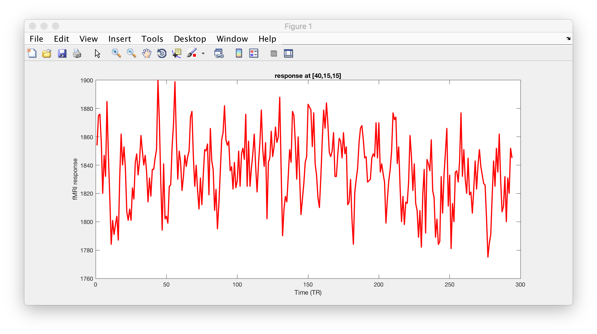
If you check back at the FSL/FEAT report for zstat1 (now you can understand why I picked that particular coordinate!), you will see the following timeseries plot.

Close, but not quite the same – What is going on here??
Adapt the following code to work with your dataset. What needs to change?
Hint 1
Data are often pre-processed. Which data is "raw", which may reflect some pre-processing?
Solutions
The data shown in the FSL/FEAT report is _not_ raw - but has been pre-processed (motion-corrected, temporally filtered, spatially blurred, ...). That intermediate data is by default stored in a nifti file called ``filtered_func_data``
% specifying path also works!
hdr_f = niftiinfo('__WIP_fMRI_SENSE_20190215100331_401.feat/filtered_func_data.nii.gz');

data_f = niftiread('__WIP_fMRI_SENSE_20190215100331_401.feat/filtered_func_data.nii.gz');

ts_f = squeeze( data_f(40,15,15,:) );  % nest, so it can go on 1 line

figure, plot(ts_f, 'r-', 'linewidth', 2)
xlabel('Time (TR)'); ylabel('fMRI response')
title('*filtered* data at [40,15,15]')

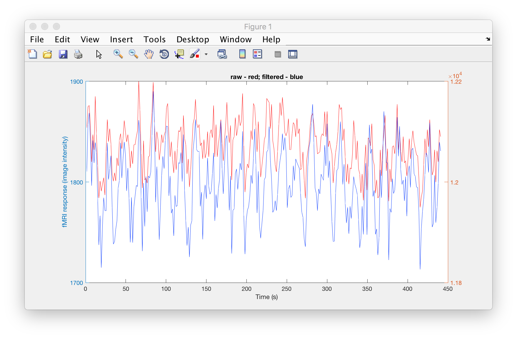
% can also look at both of them at the same times:
% but note! different y-axes
t = hdr_f.PixelDimensions(4) .* (1:numel(ts_f)); % TR -> s
figure
[AX,H1,H2] = plotyy(t, ts, t, ts_f);
set(H1,'color', [1 0 0]);
set(H2,'color', [0 0.2 1]);
title('raw - red; filtered - blue')
xlabel('Time (s)')
ylabel('fMRI response (image intensity)')

* Ninja skill
Getting the timeseries for many voxels at the same time can be done by using a loop and going through a list of indeces. A more efficient way involves using linear indexing to convert [x,y,z] triplets into one number, say, idx. If you are keen, have a look at sub2ind() and ind2sub() to see how this might work.
Linear regression
First we need to grab the design matrix from FSL/FEAT. We could copy and paste from the text file for that analysis, but there is a neater way.
I called my analysis design.fsf when I ran FEAT on the faces / objects dataset (#4). FEAT spits out the design matrix in a slightly unusual format (VEST). There is an FSL command line tool to turn it into a text file. In the Terminal:
Vest2Text design.mat design.txt
Then we can use Matlab to load the design matrix.
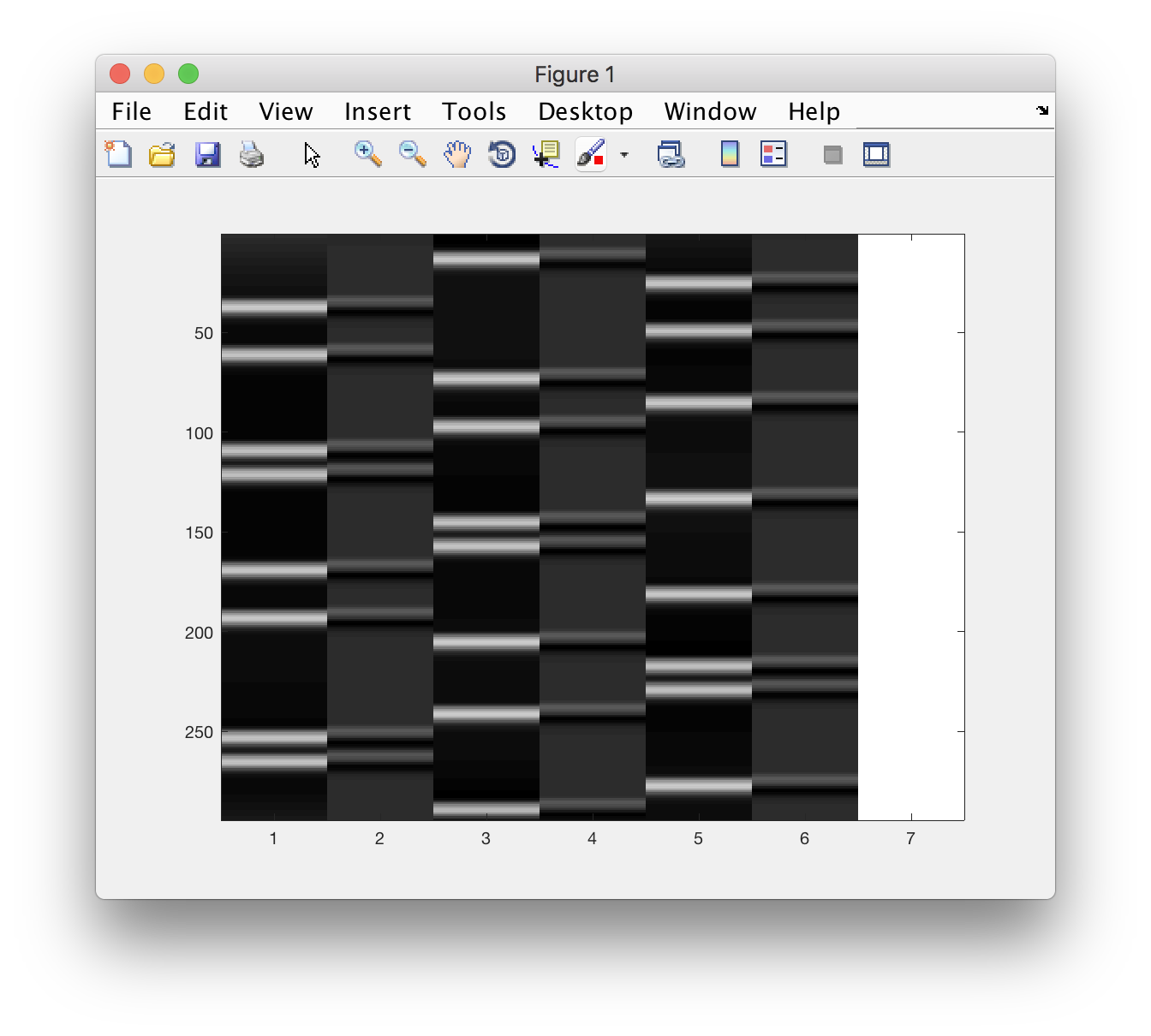
X = load('design.txt') % make sure the file is in the current folder!
% also add a column of ones!
X = [X, ones(size(X,1),1)];

% and inspect
figure, imagesc(X), colormap(gray)

And now for the linear regression:
% solve (for beta):
% data = X * \beta + \epsilon

% little gotcha... ts is INTEGERS (ask DS for nitty gritty)

ts = double(ts); % turn into normal matlab numbers

beta = X\ts;
beta_f = X\ts_f; % the filtered version
We can now think about the beta weights - but also reconstruct the best linear fit:
% model fit is beta weights times the column of X
model = X*beta; % matrix multiply!
model_f = X*beta_f;

residuals = ts - model;
residuals_f = ts_f - model_f; %just with filtered data
There is a lot more detail in the second section of the Learning Matlab pages. Also we’ll cover a little more next time.
Plot…
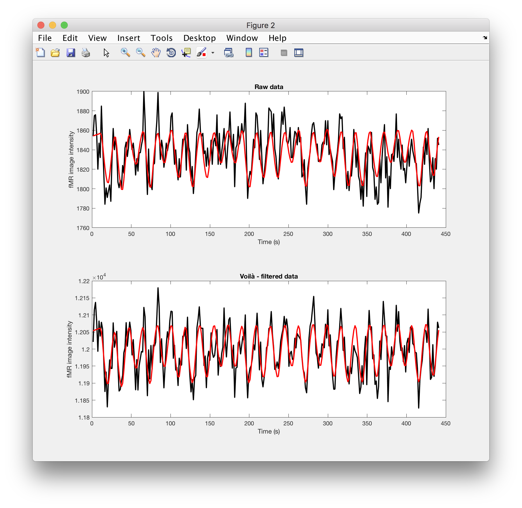
Now let’s see how close the linear prediction is to the data:
figure
subplot(2,1,1)
plot(t,ts, 'k-', t, model, 'r-', 'linewidth',2)
xlabel('Time (s)'), ylabel('fMR image intensity')
title('Raw data')

subplot(2,1,2)
plot(t,ts_f, 'k-', t, model_f, 'r-', 'linewidth',2)
xlabel('Time (s)'), ylabel('fMR image intensity')
title('Voilà - filtered data')

Notes for pre-2017b matlab
If you are trying this out in older versions of Matlab, niftiread() is not available. You could instead use the mrTools toolbox and use mlrImageReadNifti() to load NIFTI files:
which mlrImageReadNifti
% should return a valid path!
% if not, you'll need to run
addpath(genpath('/Volumes/practicals/ds1/mrTools'))