learningMatlab

Worked solution

Plotting / Fitting with a model curve

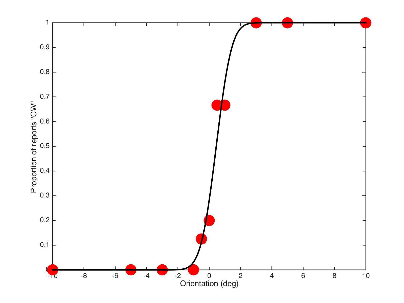
The aim is to plot and fit data to achieve something like the following:

The file summaryData.mat contains data to work with. At the command prompt, do the following:
```
load('summaryData.mat') % will load "data"
data  % find out what's in it.
```

Plot data, using the numbers in the first column as the x-values, the second column as the y-values.

figure
plot(data(:,1) , data(:,2), 'o', 'markersize',20, 'markerfacecolor', 'b')
xlabel('Orientation (deg)')
ylabel('p(CW responses)')
% and save a copy for your records
% help print
% help gcf
% ... to see why/how the following line works:
print(gcf, 'myFigure.pdf', '-dpdf')

A “nice” mathematical function / curve, that has such a shape and can be controlled with two convenient parameters is the cumulative version of the normal distribution (or Gaussian curve).

x = -10:0.2:10; % many x values -10....+10
% plot the CUMULATIVE / s-shaped function with mu=0, sigma=3
c = normcdf(x, 0, 3);
figure, plot(x, c , 'r', 'linewidth',2);
xlabel('x values'); ylabel('y values'); title('normal CDF: \mu=0, \sigma=3');

The 0 and 3 in the above example correspond to the mean (µ) and standard deviation (σ) of a normal distribution. Try plotting the CDF curve for σ = 1 (magenta curve) and σ = 5 (cyan) on the same plot. Then try changing µ, say µ = -2.5 (green) and µ = +3.4 (blue). What happens to the curves?

x = -10:0.2:10; % many x values -10....+10
% plot the CUMULATIVE / s-shaped function with other values
figure
subplot(1,2,1)
plot(x, normcdf(x, 0, 3) , 'r', 'linewidth',2);
hold on
plot(x, normcdf(x, 0, 1) , 'm', 'linewidth',2);
plot(x, normcdf(x, 0, 5) , 'c', 'linewidth',2);
title('changing \sigma')
subplot(1,2,2)
plot(x, normcdf(x, 0, 3) , 'r', 'linewidth',2);
hold on
plot(x, normcdf(x, -2.5, 3) , 'g', 'linewidth',2);
plot(x, normcdf(x, +3.4, 3) , 'b', 'linewidth',2);
title('changing \mu')

The fitting problem is: we’d like to know the “best” combination of µ and σ, such that the smooth curve they describe gets as close as possible to the data points. “Close” here means: in such a way that the squared error between the data and the corresponding points on the smooth curve is minimal… the least squares solution.
Before we can hand over the fitting to matlab we need to do the following:

we need re-wrap the normcdf function, so that it accepts the input arguments in a different order. Currently it’s: y = normcdf( x, mu, sigma ), where x are the values for which you want to find the y-values… but really we want it to be y = myNormcdf(p, x), where p = [mu, sigma] i.e. the two parameters stuck together in a list / vector. Look at the file myNormcdf.m for an example of how to do this.
we need/may want to calculate the squared error between the data (the data-y-values at each point in x) and the model/fit with a particular combination of mu/sigma (also at the corresponding x-values). Look at the file sqerror.m for an example of how to do this. The aim here is to get a single number that summarizes how close our guess of the curve is to the y-values/data. Our guess of the curve is determined by the choice of µ and σ.
just to check what that allows us to do… we can now ask for e.g. p=[0, 3.0] what is the error between that curve and the data. Next, what if I update the values to p=[1.0, 3.0]… does the error get bigger or smaller? If it gets bigger, we are moving away from a good value for p, if the error gets smaller, then the second p was better!
```
% with data loaded from summaryData!
e1 = sqerror([0, 3], data(:,1), data(:,2) )
e2 = sqerror([1.0, 3], data(:,1), data(:,2) )
% which is better??
```
the matlab function lsqcurvefit() will do this calculation internally and - by trying out many, many settings for p, find the value for it that gives the smallest possible error (the least squares solution!).

So: to put this all together now, do help lsqcurvefit to have a look at how this works in general, then try:

% with data loaded from summaryData!
bestP = lsqcurvefit(@myNormcdf, [0, 1], data(:,1), data(:,2))
% the @ in @myNormcdf is needed to make sure matlab knows you are handing it a
% function! look at "help function_handle" if you want to know more about this.
% the [0, 1] is the value for P at which you want to start the whole process
bestP =
  0.4501    0.7789

now that we have the best choice of p (stored in bestP), we can use it to calculate the curve at lots of x-values we want:

newX = linspace(-10,10, 101); % 101 values between -10 and 10
% and our myNormcdf() function is perfect for calculating these!
yFit = myNormcdf(bestP, newX);
% now plot the data and fit!
figure
plot(data(:,1) , data(:,2), 'o', 'markersize',20, 'markerfacecolor', 'b')
xlabel('Orientation (deg)')
ylabel('p(CW responses)')
hold on
plot(newX, yFit, 'k-', 'linewidth',2)

Et voilà

Back to problem description

Back to the description / problem set

This site is open source. Improve this page.